Web Rarely

Note: If you cannot view some of the math on this page, you may need to add MathML support to your browser. If you have Mozilla/Firefox, go here and install the fonts. If you have Internet Explorer, go here and install the MathPlayer plugin.

Motivation

Imagine you're building a robot that has to meet up, for purposes friendly or nefarious, with a target robot that is moving. Your robot has few sensors. It has a dead reckoning system, so it can track its own movement relative to a starting position, and it can sometimes detect the direction to the other robot, but not the distance. So at time t=0, say, the target is at a relative bearing of 90 degrees (i.e. to the right). At time t=3, it's at 87 degrees. Etc. Is it possible to compute the target's exact position, course, and speed based on such sparse information? In fact it is, and that's the idea behind target motion analysis (TMA). This has real-world uses, as the scenario described is analogous to that of a submarine tracking a target with passive sonar. Passive sonar only gives the bearing to contacts*, and a submarine crew must build a model of the world around it based on that limited information. TMA assumes that the target is moving at a fixed course and speed. Most craft take the most direct route to their destination — a straight line — so this assumption usually holds. And all that matters is that the target moves in a straight line long enough for us to gather the information needed to compute a TMA solution. Herein, I describe methods of automatically computing such solutions. I don't claim that any are state of the art, but they work and they're all much easier than doing it by hand. :-)

First let's look at some TMA examples:

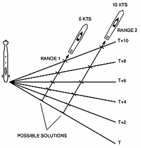
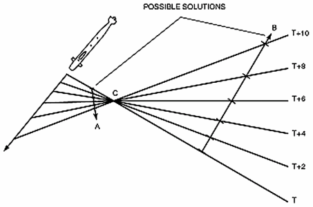
In the first image, consider a stationary submarine listening to a target. As the target moves, the submarine observes the bearing changing over time. However, this doesn't give enough information to determine a unique solution. The image shows two possibilities, but in fact there are an infinite number of possible solutions (at all different ranges). The second image shows one of the possible outcomes when both the target and observer are moving. Because the lines intersect, we know that either the two are traveling in roughly opposite directions, or they're traveling in roughly the same direction, but the sub is moving faster (which is the same thing, relatively speaking). Again, there are an infinite number of solutions. Mathematically speaking, we have to solve for four unknowns and we have six equations representing the bearing rays. The first three equations provide us with information, but further equations can be represented as linear combinations of the first three, and provide nothing new. Now consider the following:

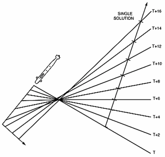
By making a turn (or by changing its speed), the submarine can obtain new lines that aren't linear combinations of the previous ones, and come up with a unique solution. This suggests a naive algorithm: simply collect the set of equations and solve them. If there's a unique solution, that's your answer. Of course, being an overdetermined system, the slightest measurement error will render the system unsolvable. But we'll look at this approach to help prepare the ground for more sophisticated approaches.

Our System

Our system will handle two kinds of observations, called bearing observations and point observations, and the observations can come from multiple observers. A bearing observation is a directional observation (e.g. from passive sonar) described by a normalized vector `b` extending from the location of the observer `o` in the direction of the bearing at time `t`. A point observation is a positional observation (e.g. from active sonar or radar) described simply by its position `p` at time `t`. The target solution is described by a point `a` (the target position at time t=0) and a velocity `v`. The target position at a given time is `a + v t`. The goal is to solve for `a` and `v`. In an ideal world, this gives a set of equations that we can solve. For point observations, we simply want to say that the target was at the observed position at the time of the observation: `a + v t = p`.

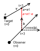For bearing observations, we want to say that the target was on the bearing ray at the time of the observation. We'll use `cross(b) * (a + v t - o) = 0`, where `cross(b)` returns a vector perpendicular to `b`. Remember that the dot product `s * t` produces a number equal to `cos(theta) |s| |t|`. So in our case, we have `cos(theta) |cross(b)| |a + v t - o| = cos(theta) |a + v t - o| = 0` (since `b` is normalized, so `|b|` and `|cross(b)|` are 1). `a + v t - o` is the vector from the observer to the target. Remember that `cos(theta)` is 1 when `theta` is 0 degrees, and 0 when `theta` is +/- 90 degrees. That is to say, the dot product of two normalized vectors is 1 when the vectors are pointing the same way and 0 when they're perpendicular (and -1 when they point in opposite directions). We want to find when the bearing vector and the actual vector to the target are pointing the same way, so we take the perpendicular vector of the bearing ray. Then, when that perpendicular vector is itself perpendicular to the vector to the target (i.e. when the original bearing vector is collinear with it), the result is zero. This causes one problem: it is zero both when the target is on the bearing ray and when it is on the reciprocal bearing ray. That is to say, it's a bearing line (in the mathematical sense) rather than a bearing ray. If both vectors were normalized, we could say `s * t = 1`, but they're not. We could also say `s * t = |t|`, but that would introduce non-linearity into the equations, making them much more difficult to solve. So we'll stick with the linear formulation for now, with the caveat that it may occasionally produce a solution on the wrong side of the observer. As a final note, remember that `b`, `o`, `p`, and `t` are constants that can be different from one observation to another. Only `a` and `v` refer to the same values across observations.

A Least Squares Solution (that almost works)

So those are the basic formulas. In the ideal case, we can simply solve them to get the solution. Geometrically, each linear equation defines a hyperplane and the solution lies at the intersection of all of the hyperplanes. If the intersection is a single point, then there is a unique solution. In reality, the system is unlikely to have a solution due to measurement and numerical error; there would be no single point where all hyperplanes intersect. A far more robust solution is to find the least squares solution to the system. Geometrically, this is the point nearest to being the intersection of all the hyperplanes. This is the first solution we'll develop. It is easy to implement, fast, and gives a solution to the problem that is the best possible (ignoring the bearing ray vs. bearing line issue described above). Incidentally, this is the approach suggested by "Dr. Sid" in this subsim.com thread which served as the inspiration and starting point for me to solve the problem myself.

In general, to find a least squares solution to a series of linear equations of the form `A x + B y + C z = D`, you first need a measure of the error in each equation, which is simply `epsilon = A x + B y + C z - D`. Then you square all the errors and add them up. For instance, `(A_0 x + B_0 y + C_0 z - D_0)^2 + (A_1 x + B_1 y + C_1 z - D_1)^2 + ... + (A_M x + B_M y + C_M z - D_M)^2`. Let's name a function `sqerr(x,y,z)` after that result. The goal is then to find the values of the parameters (`x`, `y`, and `z`) that minimize the function. It turns out this is easy to do. Because the equations are linear, squaring them produces equations that are quadratic. A quadratic formula describes a quadratic surface, in this particular case, an elliptic paraboloid (i.e. a parabola generalized to N dimensions) that I believe always opens upward. Such a paraboloid is very easy to minimize. It has one minimum which can be found by starting at any point and following the gradient downward. This can be done analytically by considering that all optima of functions occur at stationary points: points where the derivative is zero. In the case of the parabola, there is one stationary point which is a global extremum. So we can simply take the derivative of the squared error function and solve for the point where the derivative is zero.

The derivative of `sqerr(x,y,z)` as defined above is rather too long to reproduce in full, but I will note that it can be produced by considering the squared error of each linear equation independently. The derivative of the sum equals the sum of the derivatives. So we'll just look at a single representative form: `(A x + B y + C z - D)^2`. This expands into a nasty quadratic formula. Then we compute its derivative. Since the function is three-dimensional, the derivative is called the gradient and is a vector of three dimensions, of which each component is the partial derivative for the corresponding parameter:

`(del sqerr) / (del x) = 2(A^2 x + A B y + A C z - A D)`
`(del sqerr) / (del y) = 2(A B x + B^2 y + B C z - B D)`
`(del sqerr) / (del z) = 2(A C x + B C y + C^2 z - C D)`

Remember, though, that the full gradient formulas use all `M` linear equations, and so are actually like `(del sqerr) // (del x) = 2((A_0^2 + A_1^2 + ... + A_M^2)x + ...)`, although I will continue to write the shortened form. Note that although the equations for the gradient components contain seemingly non-linear bits like `A^2`, these only relate to the known constants, so we can simply compute `A^2` and get another known constant. The important thing is that it remains linear in regard to the variables. Now, to find the stationary point, we need to find the point where the gradient is a zero vector. That is the same as saying that we need to find the values of `x`, `y`, and `z` that make all three partial derivatives equal to zero. (I.e. `2(A^2 x + A B y + A C z - A D) = 0`, etc. Actually, the factor of 2 can be removed, since it doesn't affect the solution.) This gives us three linear equations, called the normal equations, which can be solved to get the least-squares solution to the original problem:

`A^2 x + A B y + A C z = A D`
`A B x + B^2 y + B C z = B D`
`A C x + B C y + C^2 z = C D`

There are many ways to programmatically solve a set of linear equations, but I won't dwell on them. Look at Gauss-Jordan elimination for a simple method. (If you just want some code, my math library supports several methods.) Now that we know how to solve a least squares problem in general, what are the exact formulas for TMA? These follow directly from the equations for our two types of observations, given above: `a + v t = p` and `cross(b) * (a + v t - o) = 0`. The only thing to do is to expand the vectors and rearrange them. For `a + v t = p`, note that this can be written as `|a + v t - p| = 0`, which expands to `sqrt((a_x + v_x t - p_x)^2 + (a_y + v_y t - p_y)^2) = 0`. This is clearly nonlinear, but when we take the squared error, the square root disappears and we're left with a quadratic again: `(a_x + v_x t - p_x)^2 + (a_y + v_y t - p_y)^2` is the squared error for a point observation, and equals the squared distance from the point. The equation for the bearing observation, `cross(b) * (a + v t - o) = 0`, expands to `b_y(a_x + v_x t - p_x) - b_x(a_y + v_y t - p_y) = 0`, and the squared error is `(b_y(a_x + v_x t - p_x) - b_x(a_y + v_y t - p_y))^2`, which equals the squared distance from the bearing line. Since the errors for both have the same unit (squared distance), we can mix the two types of observations freely. You can then sum the derivatives to get four normal equations (one per unknown – `a_x`, `a_y`, `v_x`, and `v_y`) and solve them to get the least squares solution to the TMA problem.

Constraints

It's very useful to be able to feed additional knowledge into the system to constrain the solution. For instance, if you can infer the target's speed (from experience, or via demodulated noise (DEMON) analysis) or its course (from an intelligence report) or its range, you can turn easily a TMA problem with an infinite number of solutions into one with a unique solution, and by fixing some parameters you can improve the accuracy of the least squares solution. Some constraints are easy to implement. For instance, if course and speed are known, that means `v` is known, and you can solve the same equations while treating `v` as a constant. This yields a two-dimensional problem with a vastly reduced solution space. If only course is known, that is equivalent to knowing the direction but not the length of `v`. By taking `v` to be a constant, normalized vector and introducing a scalar speed variable `s`, the equations become `a + v s t = p` and `cross(b) * (a + v s t - o) = 0`, where the unknowns are `a` and `s`, which is a three-dimensional problem. Unfortunately, constraining the speed by itself is more difficult, as the equation `|v| = s` is nonlinear (as is `|v|^2 = v_x^2+v_y^2 = s^2`). If you represent the speed directly as a constant, you can use a variable `theta` to represent the course angle, where `v_x = -sin(theta)` and `v_y = cos(theta)`, but that is also nonlinear. I don't think it's possible to constrain speed while maintaining linear equations.

When the Target Maneuvers

If the target doesn't move in a straight line, there are a few things you can do. First, if the target is simply zig-zagging or swerving along an average course, the solutions developed here will eventually converge on the average course. But if the target makes a turn and holds to the new course, that is more difficult to handle. Given a TMA solution for the original course, if the error is plotted as new measurements are collected, you can visually detect a clear point where the average error begins to increase progressively, and that is the point when the target turned. This increase in error can be detected programmatically, but it requires comparing new data against old models, and the questions of how many old models you should maintain and what thresholds to use are messy. If you can find the turning point, however, you can simply discard all older observations.

A simpler approach is to decrease the weight given to older observations. This can be done by scaling down the error associated with them. If the error from old observations becomes negligible, the solution will converge on the target's new course after a time. Although it can't snap to the new course quickly, like the previous approach, it should be more robust in general. Neither of these approaches are implemented in the solutions on this page, but the latter is a straightforward addition.

A Quadratic Programming Solution

There is one major problem with the least squares solution. As described above, it uses the bearing line rather than the bearing ray, so it can place the target on the wrong side of the observer. One way to fix this while retaining the ability to get an exact solution to the least squares problem is to use quadratic programming (QP). Quadratic programming is a set of techniques for finding an exact minimization of a quadratic form subject to linear constraints (both equality and inequality). To constrain the solution of `cross(b) * (a + v t - o) = 0` to use the bearing ray rather than the bearing line, we simply need linear constraints of the form: `b * (a + v t - o) >= 0` (one constraint per bearing line). As discussed above, the dot product of two normalized vectors is 1 when they point the same way and 0 when they're perpendicular, and -1 when the point in opposite directions. By ensuring that the dot product is greater than or equal to zero, we ensure that the vectors are pointing in roughly the same direction (i.e. the angle between them is not greater than 90 degrees). The quadratic that we would use QP to minimize would be the quadratic formed by the sum of squared errors. This would produce the exact least squares solution while ensuring it always uses bearing rays rather than bearing lines.

I implemented the quadratic programming TMA solution, but information was sparse enough and the math complicated enough that I was forced to use a third-party QP solver. I didn't like taking a dependency on an obscure, non-redistributable 20+ megabyte package for an application with a 170k executable. Also, for all its complexity, QP didn't buy me much. It only fixed an edge case. Still lacking was the ability to add speed constraints, which are the most useful kind of TMA constraint.

An Extensible Numerical Minimization Solution

I had been sticking to methods that were guaranteed to give exact solutions (like least squares and QP) and avoiding methods without such guarantees, but at this point I had few options. There are methods like quadratically constrained quadratic programming that would allow a speed constraint, but information about them is even more difficult to find than information about QP, and I couldn't find any usable third-party implementations, so I finally turned to numerical minimization. Numerical minimization generally takes a point, evaluates the function and its derivative at that point, decides where to go from there, and repeats until the derivative vanishes. The derivative can give you a downhill direction, forming the basis of the highly versatile Newton's method, but outside of toy problems it is very difficult to find the global minimum of a general nonlinear multidimensional function. Even finding local minima requires finesse. That said, after trying several four-dimensional formulations that didn't work well due to the existence of many local optima, I developed a five-dimensional formulation that happens to be globally convergent from nearly any starting point (at least in the tests I've done so far), and to which various constraints can be added.

The function again computes the sum of squared errors. `sqerr(a_x,a_y,d_x,d_y,s)` is a function of 5 variables, similar to the formulations above. `a` is the target's initial position, `d` is a normalized direction vector, and `s` is its speed. The function computes the error pretty much as above. It uses `a + d s t = p` and `cross(b) * (a + d s t - o) = 0` for point and bearing observations, respectively. In case a target would be on the wrong side of the observer, it uses `a + d s t - o` (the distance from the observer) as the error. In other words, for point observations it uses the distance to the point, and for bearing observations, it uses the distance to the bearing ray. By itself, it is possible to minimize this function and get a good result. Now, without constraints, it will almost certainly end up that `d` is not normalized, that `s` is negative, etc. but multiplying `d` by `s` will still give you the correct velocity vector. In pseudocode:

# computes the squared error in a TMA solution represented by variables a, d, and s, where a is the target's initial
# position, d is the target's normalized direction vector, and s is the target's speed
function sqerr(a, d, s) :=
    squaredError = 0

    for each point observation P
        targetPoint = a + d * s * P.time
        squaredError += (targetPoint.x - P.x)^2 + (targetPoint.y - P.y)^2
    end for

    for each bearing observation B
        targetPoint = a + d * s * B.time
        observationVector = targetPoint - B.observerPoint
        # calculate the distance to the bearing ray by taking the distance from the line if the target would be on the
        # correct side of the observer, and the distance to the endpoint if the target would be on the wrong side
        if dotProduct(B.bearingVector, observationVector) >= 0 # if the target would be on the correct side of the observer...
            squaredError += dotProduct(B.bearingVector.crossVector, observationVector)^2
        else # if the target would be on the wrong side of the observer...
            squaredError += (targetPoint.x - B.observerPoint.x)^2 + (targetPoint.y - B.observerPoint.y)^2
        end if
    end for

    return squaredError
end function

Adding constraints to the function uses the following fact: if you want to minimize a general function `f(x)` subject to general constraints `c(x) <= 0`, then the problem is equivalent to performing unconstrained minimization of a new function `g(x) = f(x) + r p(c(x))` in the limit as `r -> oo` or `r -> 0` (depending on the method), where `p(e)` converts a measure of the degree of constraint violation `e` into a penalty value and `r` is a factor that scales the penalty up or down. This general technique is known as using a penalty method or a barrier method, depending on the exact formulation. In a penalty method, `r` starts low (yielding a small penalty) and increases over several iterations, resulting in increasing conformance to the constraints as the unconstrained minimizer must pay more attention to the increasing penalty for constraint violation. The penalty method does not prevent violation of constraints, however; it only penalizes them. A barrier method, on the other hand, uses as its function `p(e)` something that contains a singularity as `e` approaches zero, such as `-log(-e)` or `-1//e`. At the singularity, the penalty rises to infinity, preventing constraints from ever being violated. However, it penalizes the minimizer for even getting close to violating a constraint. That is to say, it penalizes perfectly valid points, which is why the correct solution is found by taking `r -> 0`, where the distortion applied to those valid points gradually vanishes.

There are pros and cons to both approaches. Imagine that the inequality `c(x) <= 0` defines a region of space where the constraints hold. This is called the feasible region and points are said to be feasible if they satisfy the constraints. With the penalty method, the process can potentially produce results that violate the constraints, but is capable of navigating areas of the search space outside the feasible region, and the process can be started from any point. With the barrier method, the process can never leave the feasible region. This restricts its possible movement, and requires that the initial point satisfy the constraints. If the barrier divides the space into separate subspaces, the process won't escape the subspace containing the initial point, so if the minimum resides in another subspace, it won't be found. The barrier method is also generally unsuitable for equality constraints, as the penalty would almost always be infinite. Despite the barrier method's apparent limitations, when it works it works quite well, usually producing good results with much less computational effort than penalty methods.

This theory allows us to take a general unconstrained function minimizer and layer constraints on top of it in an extensible way, without needing to modify the original function that we're minimizing. Given a general function minimizer that finds a local minimum of a function, you can use it to minimize `g(x)` repeatedly while increasing or decreasing `r` steadily depending on whether you use a penalty or barrier method (say starting from 1 and increasing or decreasing by a factor of 10 each iteration) until one of three things occurs:

• The fraction of the function's value that came from penalties was less than a given amount: `p(c(x)) // |g(x)| < epsilon_1`.
• The parameters have largely stopped changing: `|x - oldx| < epsilon_2`.
• The value has largely stopped changing: `|g(x) - oldValue| < epsilon_3`.

In the context of TMA, I'm using a penalty method, primarily because I need to support equality constraints (e.g. speed is 5 knots). Specifically, I'm using a quadratic penalty method, where `p(e) = max(0,e)^2`. This defines a penalty of zero inside the feasible region, and a rapidly increasing penalty outside it. Now how do you go about writing `c(x)`? Well, as an example, to add an equality constraint (i.e. `x=a`) you can return `|x-a|`. A bounds constraint (i.e. `a <= x <= b`) can be `max(a-x, x-b)`. If you have multiple constraints, you can use `g(x) = f(x) + r_0 p(c_0(x)) + r_1 p(c_1(x)) + ... + r_n p(c_n(x))`. This allows each constraint to have its own weight, although you can also just use a single value of `r`.

Now I'll describe the constraints I use. First is a speed range. Since the speed is a separate variable in my formulation, that is simply a bounds constraint as described in the previous paragraph. (Even if no speed constraint is requested, I always add one to ensure that the speed is non-negative.) Next is the normalization constraint, which ensures that `d` remains normalized. This is simply `|d_x^2 + d_y^2 - 1|` — essentially an equality constraint keeping the squared length of the vector at unity. More difficult is the course constraint. I allow a range, so you can say that the target has a course between 30 and 60 degrees, say. First, I'll note that a vector's direction can be computed as `cos^-1(v_x // |v|)` if `v_y >= 0` and `2pi - cos^-1(v_x // |v|)` if `v_y < 0`. The constraint then is simply a bounds constraint on the vector's direction. (One caveat is that we want to treat the range "between 350 and 10 degrees" differently from "between 10 and 350 degrees".) These constraints are highly non-linear piecewise functions, but when you have a general function minimizer you can do that. :-)

Everything so far has been rather simple, assuming we have one of those magical general function minimizers handy. Now we have to start developing the general function minimizer. This leads to the requirement that `g(x)`, which means `sqerr(x)` and all of the constraints, must be differentiable. This is necessary because general function minimization requires knowing which direction is downhill from a given point, and that requires the gradient. (It is possible to estimate the gradient by taking several samples around a point and seeing which way the slope is going, but that is slow and inaccurate.) So we must now define the gradient functions for all of the above. They needn't be smooth, though. They can be like `abs(x)`, which is a piecewise function differentiable everywhere except at the points where the pieces meet, and that's usually good enough. The method for computing the gradient of `sqerr()` was given in the linear squares section, and applies equally well here. So we need only compute the gradients of the constraints.

In general, a bounds constraint `c(x) = {(a-x, "if " x<=a), (x-b,"otherwise"):}}` has the derivative `c'(x) = {(-x', "if " x<=a),(x',"otherwise"):}}`. An equality constraint `c(x)=|x-a|` has the derivative `c'(x) = {(x',"if " x-a >= 0),(-x',"otherwise"):}}`. The derivative of the speed variable is simply 1 (as is the derivative of any bare variable), so the derivative of the speed constraint returns 1 or -1 as appropriate. The gradient for `d_x^2 + d_y^2 - 1` is `(2d_x,2d_y)`, so the gradient of the normalization constraint is `(2d_x,2d_y)` or `(-2d_x,-2d_y)` as appropriate. This leaves the course constraint. The derivative of `dir(v) = cos^-1(v_x//|v|)` is pretty hairy:

`(del dir) / (del v_x) = -(-v_x^2/(v_x^2+v_y^2)^(3//2) + 1/|v|) / sqrt(1 - v_x^2/(v_x^2+v_y^2))`     `(del dir) / (del v_y) = (v_x v_y) / ((v_x^2+v_y^2)^(3//2) sqrt(1 - v_x^2/(v_x^2+v_y^2)))`

These need to be negated in the case that `(v_y < 0)` or the computed angle is less than the minimum, but not both. (One condition negates it. Two conditions negate it twice, leaving it unchanged.)

The derivative of the general function `g(x) = f(x) + r p(c(x))` is simply `g'(x) = f'(x) + r c'(x) p'(c(x))`. Since I'm using a quadratic penalty method, this works out to `g'(x) = f'(x) + {(0,"if " c(x)<=0),(2r c(x) c'(x),"otherwise"):}}`. To put it all together we only need a general unconstrained function minimizer. That could occupy a whole article of its own, and I'm quite tired now. I'll only say that the BFGS algorithm works quite well, and that everything has been implemented in my math library as the class ConstrainedMinimizer, and that the solution as applied to target motion analysis has been implemented in my project Maneubo, which aims to provide a kind of virtual maneuvering board where these types of calculations can be carried out. I may have hurried through the later sections of this article, but if you're interested in more details, feel free to contact me and I'd be glad to elaborate. If you're the kind of person who benefits more from seeing actual source code rather than an abstract description (like me), feel free to browse the source code of the projects I've mentioned or to ask me for pointers to code snippets.

* A number of technologies have been developed to overcome this. The most common is the use of a towed array, which is a hydrophone (i.e. sonar sensor) or series of them towed on a very long cable behind the boat. This can allow the submarine to get bearings from multiple points (itself and a point 1000m behind it, say), and by intersecting the two bearing rays, an estimate of the target position can be found. If the towed array has many small hydrophones, beamforming techniques can be used. A more recent and advanced technology uses so-called Wide Aperture Arrays (WAA) that can provide limited distance measurement for nearby contacts. I believe it works by measuring Doppler shift and/or timing differences between collinear sensors. None of these are full solutions, since for targets that aren't nearby, the differences in measurements between the sensors will be small enough to be swamped by measurement error, but the extra observations can feed a TMA system which can pick out the statistical correlations over time.